import openeo
import xarray
import matplotlib.pyplot as pltopenEO Basics: How to load a data cube from a data collection?
This notebook provides a detailed guide on how to load a DataCube from a data collection. Additionally, it will cover how to authenticate in order to process and download data.
Setup
Import the openeo package and connect to the Copernicus Data Space Ecosystem openEO back-end.
connection = openeo.connect(url="openeo.dataspace.copernicus.eu")
connection
<Connection to 'https://openeo.dataspace.copernicus.eu/openeo/1.2/' with NullAuth>Note the NullAuth in the representation of the connection, which indicates that we are not logged in yet.
The canonical way to log in is using the authenticate_oidc() method. This might, depending on your situation, trigger an authentication procedure. Follow the instructions, if any.
connection.authenticate_oidc()Authenticated using refresh token.<Connection to 'https://openeo.dataspace.copernicus.eu/openeo/1.2/' with OidcBearerAuth>Note that the connection is now authenticated now through OidcBearerAuth.
Data Loading
With our authenticated connection, we can now start loading a data collection data to build a DataCube, filtered according to specific spatio-temporal constraints:
s2_cube = connection.load_collection(
    "SENTINEL2_L2A",
    temporal_extent=("2022-05-01", "2022-05-30"),
    spatial_extent={
        "west": 3.20,
        "south": 51.18,
        "east": 3.25,
        "north": 51.21,
        "crs": "EPSG:4326",
    },
    bands=["B04", "B03", "B02"],
    max_cloud_cover=50,
)

scl = connection.load_collection(
    "SENTINEL2_L2A",
    temporal_extent=("2022-05-01", "2022-05-30"),
    spatial_extent={
        "west": 3.20,
        "south": 51.18,
        "east": 3.25,
        "north": 51.21,
        "crs": "EPSG:4326",
    },
    bands=["SCL"],
    max_cloud_cover=50,
)

mask = scl.process("to_scl_dilation_mask", data=scl)

masked_cube = s2_cube.mask(mask)
Let’s download this slice of data in netCDF format to give it an initial inspection.
masked_cube.download("load-raw.nc")Quick visualisation of first and last observation in the timeseries.
ds = xarray.load_dataset("load-raw.nc")
# Convert xarray DataSet to a (bands, t, x, y) DataArray
data = ds[["B04", "B03", "B02"]].to_array(dim="bands")

fig, axes = plt.subplots(ncols=2, figsize=(8, 3), dpi=90, sharey=True)
data[{"t": 0}].plot.imshow(vmin=0, vmax=2000, ax=axes[0])
data[{"t": -1}].plot.imshow(vmin=0, vmax=2000, ax=axes[1]);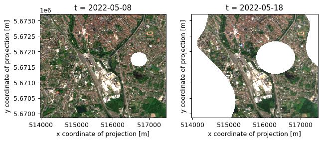
Notice how the observation on the right suffers from clouds and cloud shadows.
Data Processing
Let’s include a bit of extra data processing. We’ll build a naive composite image by taking the temporal maximum:
composite = s2_cube.max_time()Download this composite and visualize it:
composite.download("load-composite.nc")ds = xarray.load_dataset("load-composite.nc")
# Convert xarray DataSet to a (bands, x, y) DataArray
data = ds[["B04", "B03", "B02"]].to_array(dim="bands")
fig, ax = plt.subplots(ncols=1, figsize=(4, 4), dpi=90)
data.plot.imshow(vmin=0, vmax=2000, ax=ax)